Data has become an integral part of decision making for businesses. Therefore Quality Data is paramount to ensure that stakeholders are making accurate conclusions.
Bad data can lead to significant financial losses. Gartner estimates that every year, poor data quality costs organizations an average of $12.9 million.
This is why Data Cleaning is an important part of Data Analysis.
Failing to clean your data can lead to inconsistent results, which may negatively impact your business decisions. Accuracy in data analysis is a crucial factor for running a successful, data-driven business.
In this blog, I’ll show you how to clean data in Google Sheets using various formulas and built-in tools.

Why Data Cleaning Is Important
When you receive raw data from your client, databases, or external sources, it’s not always in a standardized format. There are some issues you need to address before using your data for analysis. Like typos, whitespace, inconsistent formats, null values, or duplicate data.
Data cleaning helps you ensure to solve these problems and make your dataset accurate, consistent, and ready for analysis.
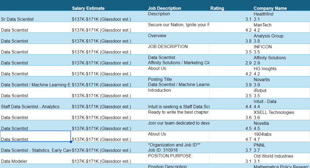
Now we will walk through the problem of cleaning a dataset in Google Sheets. For this we will download a dataset from Kaggle which is about Data Science Job Posting on Glassdoor.
We will first identify issues and fix them one by one using formulas or built-in features to fix them.
Import the Dataset
Start by importing your dataset into Google Sheets.
You can import a CSV or Excel file by going to File > Import.

Identify Issues Before Cleaning
The first step in cleaning data in Google Sheets is to get an overview of your dataset.
- Review column names and data types.
- Look for missing values or placeholders (e.g., “NA”).
- Check for duplicates or inconsistent formatting.
Take your time to identify these issues upfront. It will ensure you apply the correct cleaning methods.

Make a copy of the dataset
Before making any changes, always create a copy of your dataset. This ensures you can revert to the original if needed.
To duplicate the dataset in Google Sheets:
- Right-click on the tab containing the dataset.
- Select Duplicate.

Now that our dataset is ready, we can begin the data cleaning process. It’s important to note that Google Sheets offers several built-in features that allow you to make changes to your data without needing to use formulas. We’ll go through these features one by one.
Remove Duplicates
Google Sheets has a simple tool to remove duplicates. This is a key step when cleaning data, as duplicates can skew your analysis.
Go to: Data > Data Cleanup > Remove Duplicates.
This ensures that each row of data is unique, preventing errors caused by repeated data.

Handle Missing Values
Missing values can disrupt your analysis, so it’s important to address them. You have two main options:
1) Highlight missing values: Use Conditional Formatting to highlight empty cells by going to Format > Conditional Formatting and setting it to fill empty cells with a color.

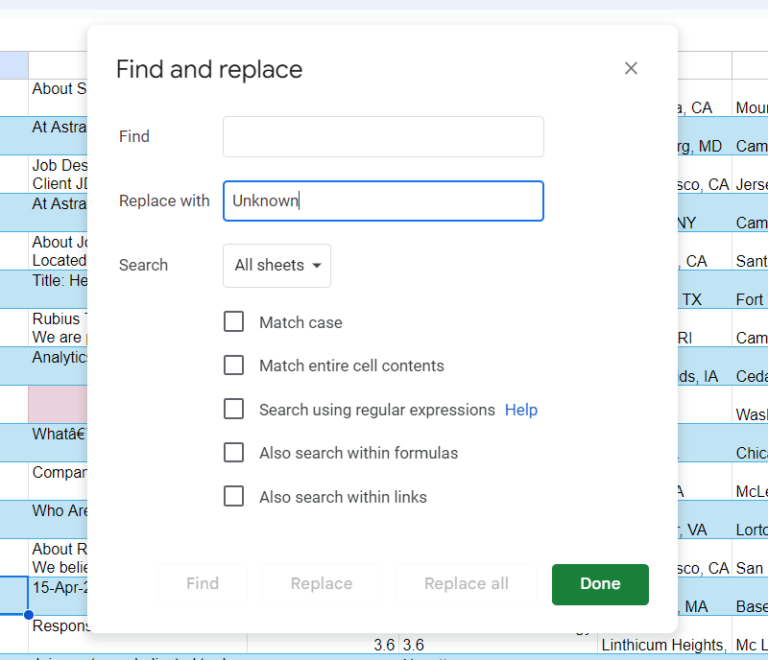
2) Replace missing values: If needed, replace empty cells with a placeholder like “Unknown” using Find and Replace.
Use: Ctrl + F and then click Replace All.

Trim Whitespace
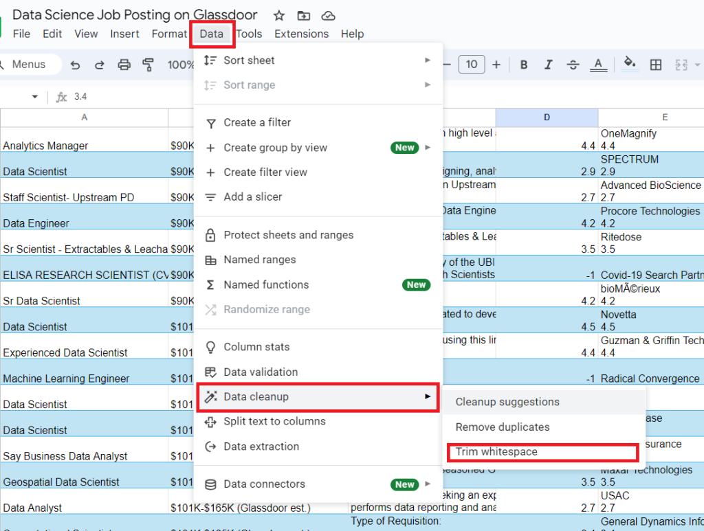
Unnecessary spaces in your data can cause errors in formulas or disrupt sorting. Use Google Sheets’ built-in feature to remove extra spaces:
Go to Data > Data Cleanup > Trim Whitespace.
This removes all leading, trailing, and extra spaces between words or numbers, ensuring your data is clean.

Using Formulas to Clean Data
SEARCH and IFERROR: Categorizing Job Titles
Starting from the first column we can see that the header of the 1st column is missing. So we will give it a name like “Job Title” as you can see that this column lists all the job titles that companies are looking for in the field of data science.
But there are so many different job titles listed, so we are going to categorize them using SEARCH and IFERROR functions. Here’s an example formula to group titles like “Data Scientist,” “Data Analyst,” and “Business Intelligence Analyst.”
=IFERROR(IF(SEARCH("Data Scientist", A2), "Data Scientist", IFERROR(IF(SEARCH("Business Intelligence Analyst", A2), "Business Intelligence Analyst", IFERROR(IF(SEARCH("Data Analyst", A2), "Data Analyst", IFERROR(IF(SEARCH("Data Engineer", A2), "Data Engineer", "Unknown"))))))) This formula searches for specific job titles and standardizes them. If none are found, it returns “Unknown.”

SUBSTITUTE: Cleaning Salary Estimates
In the 2nd column “Salary Estimate” we are going to clean this column by removing unnecessary text like “(Glassdoor est.)” or “(Employer est.).” For this we will use the SUBSTITUTE function:
=SUBSTITUTE(SUBSTITUTE(C2, " (Glassdoor est.)", ""), " (Employer est.)", "")
This formula removes those extra phrases, leaving only the salary range.

ISNUMBER: Identifying Key Skills
Next, we’ll focus on the ‘Job Description’ column, which provides detailed information about the job. If you look clearly it mentions key tools and skills like Excel and Python.
We will now extract the tools mentioned in the job descriptions, including Excel, Tableau, Power BI, Python, Spark, and others, and create a new column for each tool to track their presence.
=IF(ISNUMBER(SEARCH("Excel", F2)), "Yes", "No") This checks if “Excel” is mentioned and returns “Yes” if it’s found and “No” if it’s not.
You can create similar formula for other tools.

TRIM & REGEXREPLACE: Cleaning Company Names
Next, we’ll move to the ‘Company Name’ column. In this column, you’ll notice that the company names are often listed with a rating, such as ‘Healthfirst 3.1.‘
Since there’s already a separate column for ratings, we will remove the rating from the company name using REGEXPREPLACE function to keep the data clean.
=TRIM(REGEXREPLACE(P2, "\s*\d+(\.\d+)?$", ""))
This formula removes any number at the end of the company name, leaving only the name itself.

LEFT & RIGHT: Splitting Location Data
The column “location” includes both city and state (e.g., “New York, NY”). We will split it into two separate columns:
For City:
=IF(ISNUMBER(FIND(",", R2)), LEFT(R2, FIND(",", R2)-1), "") For State:
=IF(ISNUMBER(FIND(",", R2)), RIGHT(R2, LEN(R2)-FIND(",", R2)-1), "") 
SUBSTITUTE and SEARCH: Cleaning Employee Size Data
To clean employee size data (e.g., “51 to 200 employees”), we will use the SUBSTITUTE function:
=IF(ISNUMBER(SEARCH("to", X2)), SUBSTITUTE(SUBSTITUTE(X2, " employees", ""), " to ", "-"), SUBSTITUTE(X2, " employees", "")) This formula converts “51 to 200 employees” into “51-200.” And “1000+ employees” to “1000+.”

TRIM and MID: Standardizing Ownership Types
For “Type of Ownership” column (e.g., “Company – Public”), we will simplify the data using the formula:
=TRIM(IF(ISNUMBER(SEARCH("Company -", AA8)), MID(AA8, FIND("-", AA8) + 1, LEN(AA8)), IF(ISNUMBER(SEARCH("Nonprofit Organization", AA8)), "Nonprofit", "Unknown"))) This extracts the relevant information and standardizes it.

TEXT: Formatting Revenue Data
In the ‘Revenue’ column, the company’s revenue is listed, but we want to simplify these details. For example, if it says ‘$100 to $500 million (USD)’, we will display it as ‘$100-$500 M‘.
If ‘billion’ is mentioned, we’ll convert it to ‘B’. And, for any cell where ‘Unknown‘ or ‘Non-Applicable‘ is listed, we’ll simply write ‘Unknown’.
This process is similar to what we did with the ‘Size of Employees’ column, where we replaced ‘to’ with a hyphen and removed unnecessary text like ’employees’. We’ll apply a similar approach here.
=IF(AND(ISNUMBER(SEARCH("million", AE17)), ISNUMBER(SEARCH("billion", AE17))), "$"&TEXT(LEFT(AE17, FIND(" million", AE17)-1)/1000, "0.0")&"-"&TEXT(MID(AE17, FIND("to $", AE17)+4, FIND(" billion", AE17)-FIND("to $", AE17)-4), "#")&" B", IF(ISNUMBER(SEARCH("million", AE17)), SUBSTITUTE(SUBSTITUTE(AE17, " million (USD)", " M"), " to ", "-"), IF(ISNUMBER(SEARCH("+ billion", AE17)), SUBSTITUTE(SUBSTITUTE(AE17, " billion (USD)", " B"), "+", "+"), "Unknown"))) This formula converts the salary data into a standardized format like “$0.5-$1 B.”

Final Cleanup and Formatting
- In some cells, the value “-1” indicates missing data. You can easily replace “-1” with “Unknown” to clarify this in your dataset.
- We have left some columns unformatted, as no changes were needed.
- To quickly apply a formula to an entire column, you can use the shortcut Ctrl + Shift + Down Arrow to select the column, and then press Ctrl + D to copy the formula down to all selected cells.
With these steps your dataset should be clean and consistent. Always double-check your data for any missed issues, and make sure to document your cleaning steps for transparency.

